Rhomboid Bifiltration (multicover)

The Rhomboid Bifiltration is a topologically equivalent bifiltration to the multicover bifiltration, introduced in [Computing the Multicover Bifiltration], whose code is available here.

import numpy as np
import gudhi as gd
import multipers as mp
import matplotlib.pyplot as plt

Definition

Let \(P\) be a point cloud in some metric space \((X,d)\). The multicover bifiltration is the bifiltration \(F\) indexed over \(\mathbb{R} \times \mathbb{N}^{\mathrm{op}}\), defined as follows:

\[\begin{align*} \forall (r,k)\in \mathbb{R} \times \mathbb{N}^{\mathrm{op}}, \quad & F_{r,k}=\bigcup_{\substack{i_1, \dots, i_k\\ \forall j_1\neq j_2, i_{j_1} \neq i_{j_2}}} \bigcap_{j=1}^k B(p_{i_j}, r)\\ &= \left\{ x\in X \mid \exists k \textnormal{ distinct points } (p_i)_{1\le i \le k} \in P, \textnormal{ s.t. } \max_i d(p_i, x)\le r\right\} \end{align*}\]

Note that this filtration is not 1-critical/free. The Rhomboid Tiling bifiltration is a topologically equivalent 1-critical bifiltration, that we do not develop here.

We identify \(\mathbb N^{\mathrm{op}}\) with \(-\mathbb N\).

A first example

np.random.seed(0)
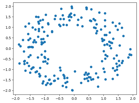
x = mp.data.noisy_annulus(200,0, dim=2) # dataset
plt.scatter(*x.T)
k_max = 50 # the maximum of ball intersection to look at
degree=1 # homological degree

s = mp.filtrations.RhomboidBifiltration(x, k_max=k_max, degree=degree, verbose=True)
len(s)

[rhomboid_tiling] backend=rhomboid_tiling mode=cpp_interface degree=1 k_max=50
[multipers.rhomboid][timing] points_to_kernel=1.85e-05s rhomboid_core=12.5069s interface_convert=0.107938s total=12.6149s bifiltration_cells=5218781 output_cells=4357848
[rhomboid_tiling][Done (13.213s)] cpp_call=13.213s

4357848

This filtration is very large in general ; before computing an invariant it is generally recommended to simplify it, via a sequence of squeezes or minimal presentations.

multicover = (s
    .grid_squeeze(
        resolution=200, # coarsens the filtration grid
        strategy="regular_closest", 
        threshold_min=[0, -k_max], # thresholds the filtration values
        threshold_max=[4, 0],
    )
    .minpres(degree) # mpfree
    .astype(vineyard=True) # for mma
)
len(multicover)

78032

Hilbert Function

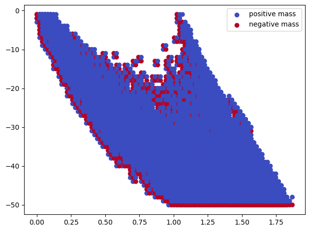
The signed barcodes of this filtration are not very readable

sm, = mp.signed_measure(multicover, degree=degree, plot=True);

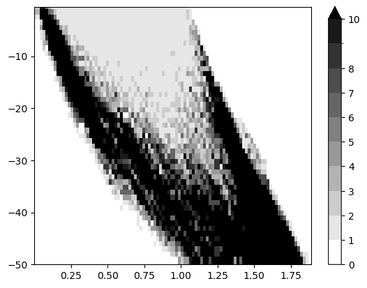
The induced Hilbert function suggest a significant cycle

mp.point_measure.integrate_measure(*sm, plot=True);

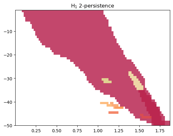
Module approximation

mod = mp.module_approximation(multicover, n_jobs=10)
mod.plot()

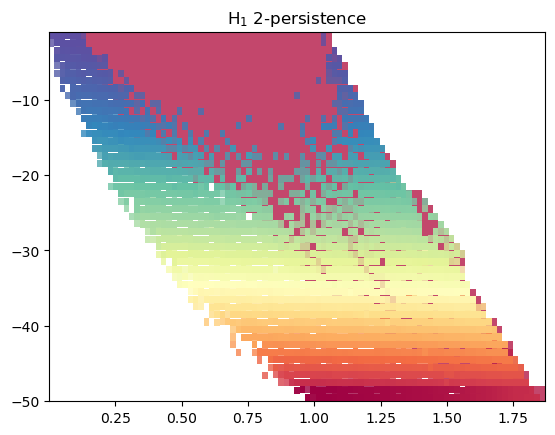
This is a bit bloated, so we can just plot the summand larger than a given threshold. We clearly recover the inital cycle here.

mod.plot(min_persistence = .1)

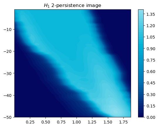
Another alternative is to look at a representation of MMA, which weights the summands w.r.t. their “size”.

mod.representation(plot=True, degrees=[1]);

Scaling

As far as I tested, this filtration doesn’t scale much more than with a few hundreds of points.