Degree Rips bifiltrations

import numpy as np
import gudhi as gd
import multipers as mp
import matplotlib.pyplot as plt

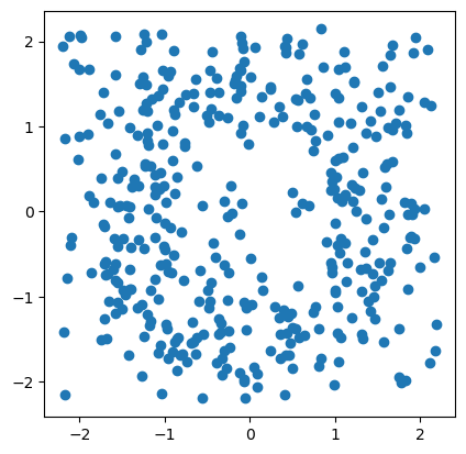
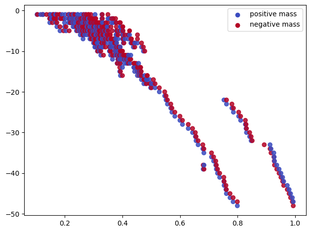
Let start with a noisy dataset, and let’s try to recover some topological signal.

np.random.seed(0)
X = mp.data.noisy_annulus(200,200)
plt.scatter(*X.T);plt.gca().set_aspect(1)

Definition

Now, if \(\mathrm{Rips}_t(X)\) is the Viertoris-Rips filtration at scale \(t\ge 0\), then \(\mathrm{DegreeRips}(X)\) is a bifiltration over \(\mathbb{R}_+\times \mathbb{N}^{\mathrm{op}}\), defined as follows:

\[\mathrm{DegreeRips}_{r,k}:= \left\{ \sigma \in \mathrm{Rips}_r \mid \forall x\in \sigma,\, \mathrm{degree}(\textnormal{1-skeleton}(\mathrm{Rips}_t(X)),x)\ge k\right\},\]

where given a graph \(G\) and a node \(n\), \(\mathrm{degree}(G,n)\) is the degree of the node \(n\) in \(G\).

Note that this filtration is not 1-critical. See TODO for more details.

TODO : example.

# DegreeRips uses 1-based degree indexing, so we start at 1.
degrees = np.arange(1, 51, dtype=int)
# The associated DegreeRips filtration can be encoded in a (multicritical) simplextree
st_multi = mp.filtrations.DegreeRips(points = X, ks=degrees,threshold_radius=1.5)

This simplextree st_multi only holds the 1-skeleton of this bifiltration. It can be extended, as usual, to a higher dimension complex.

print(len(st_multi))
st_multi.expansion(2)
print(len(st_multi))
st_multi.prune_above_dimension(1)
print(len(st_multi))

23548
669199
23548

First invariant computation

As shown above expanding simplextree without having access to edge collapse algorithms, or a similar preprocessing step, this is not tractable.

A simple strategy to compute invariants that only rely on 1-d slices is simply to lazy expand them once they are pushed forward on a line, and 1-d collapsed. This can be achieved using the expand_collapse flag in mp.signed_measures.

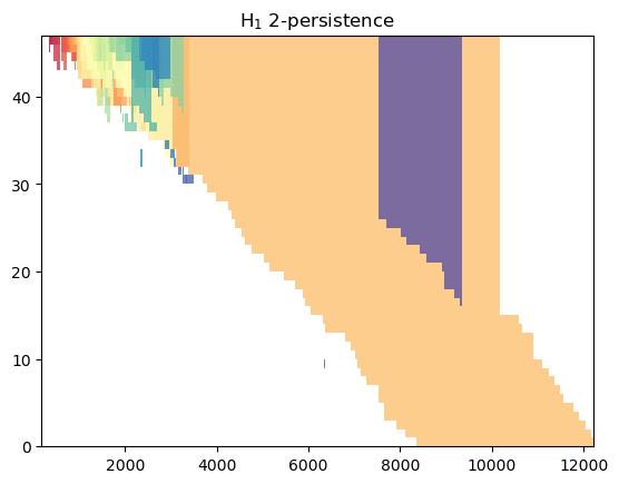
sm0,sm1 = mp.signed_measure(st_multi, degrees=[0,1], invariant="hilbert", plot=True, expand_collapse=True);

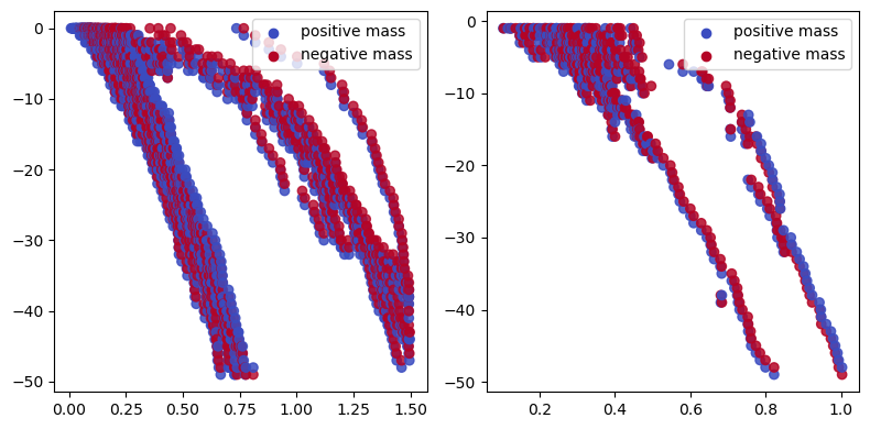
The hilbert signed measure encodes the hilbert function, from which we clearly see the 1-cycle here.

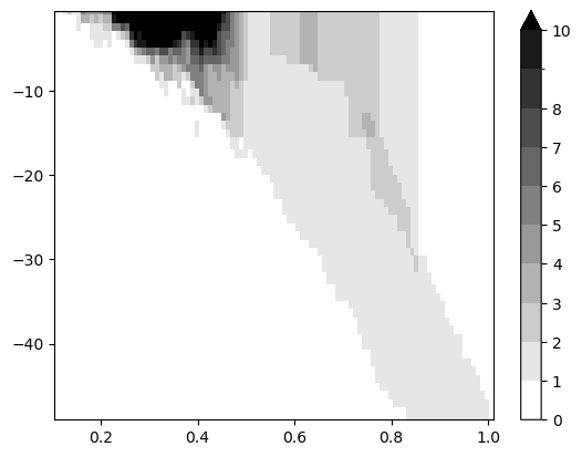
mp.point_measure.integrate_measure(*sm1, plot=True);

Coarsenning strategies

Invariants that cannot use this strategy cannot be computed in a reasonable time without premilitary preprocessing (WIP) or filtration approximations. Degree 0 is not affected as it doesn’t require any expansion.

MMA computations involving a geometric axis (here rips) can be computed more efficiently on the [1,0] direction (although the recovery guarantees change), with the second coordinate swapped (which, in this case, guarantees a “generic initialization”).

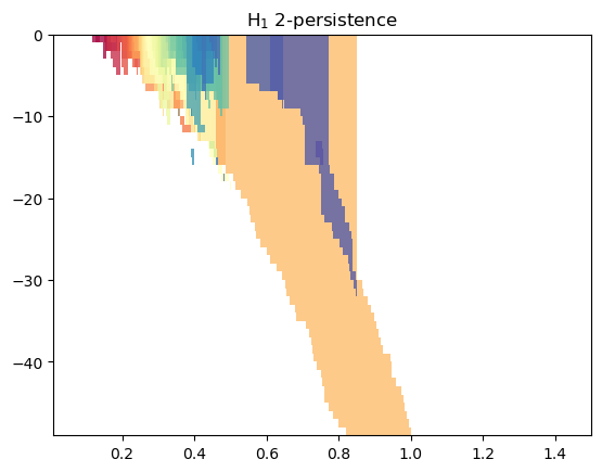
st_multi.expansion(2)
mod = mp.module_approximation(st_multi, direction=[1,0], swap_box_coords=[1], from_coordinates=True)
mod.plot(1)

/Users/dlapous/micromamba/envs/313/lib/python3.13/site-packages/multipers/logs.py:115: GeometryWarning: Got a degenerate direction. This function may fail if the first line is not generic. 
Set `multipers.logs.GeometryWarning.enabled = False` to disable this warning.
  _emit("geometry", message, stacklevel=stacklevel)
/Users/dlapous/micromamba/envs/313/lib/python3.13/site-packages/multipers/logs.py:115: GeometryWarning: Squewed filtration detected. Consider rescaling the filtration for interpretable results.
  _emit("geometry", message, stacklevel=stacklevel)

A first strategy is to approximate the Rips itself, using, e.g., a sparse rips. Note that this is not backed up by theoretical guarantees.

# A custom complex (gudhi simplextree) can be put there instead.
st = gd.RipsComplex(points=X, max_edge_length=1).create_simplex_tree()
st = mp.filtrations.DegreeRips(simplex_tree=st, ks=np.arange(1, 50, dtype=int))

st_dim2 = st.copy()
st_dim2.expansion(2)
len(st_dim2)

190779

s = mp.Slicer(st_dim2)
mp.signed_measure(s, degree=1, plot=True)
len(s)

190779

One-criticalify

Multi-critical filtrations can be represented by one-critical filtrations, by following [Combinatorial presentation of multidimensional persistent homology], which was later improved to allow computing free resolutions of chain chain complexes [https://arxiv.org/abs/2512.08652], whose code is available [here] and needs to be installed.

one_critical = mp.ops.one_criticalify(s)

d1 = one_critical.minpres(1)

mp.module_approximation(d1).plot()

TODOs to make it tractable

WIP