Point Cloud Optimization

import multipers as mp
from multipers.data import noisy_annulus, three_annulus
import gudhi as gd
import numpy as np
import matplotlib.pyplot as plt
import torch
# t.autograd.set_detect_anomaly(True)
from multipers.plots import plot_signed_measures, plot_signed_measure
from tqdm import tqdm
torch.manual_seed(1)
np.random.seed(1)

Spatially localized optimization

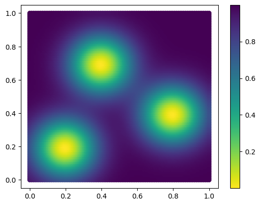
The goal of this notebook is to generate cycles on the modes of a fixed measure.

In this example, the measure is defined (in the cell below) as a sum of 3 gaussian measures.

## The density function of the measure
def custom_map(x, sigma=.17, threshold=None):
    if x.ndim == 1:
        x = x[None,:]
    assert x.ndim ==2
    basepoints = torch.tensor([[0.2,0.2], [0.8, 0.4], [0.4, 0.7]]).T
    out = -(torch.exp( - (((x[:,:,None]- basepoints[None,:,:]) / sigma).square() ).sum(dim=1) )).sum(dim=-1)
    return 1+out

x= np.linspace(0,1,100)
mesh = np.meshgrid(x,x)
coordinates = np.concatenate([stuff.flatten()[:,None] for stuff in mesh], axis=1)
coordinates = torch.from_numpy(coordinates)
plt.scatter(*coordinates.T,c=custom_map(coordinates), cmap="viridis_r")
plt.colorbar()

<matplotlib.colorbar.Colorbar at 0x7f7c733a8980>

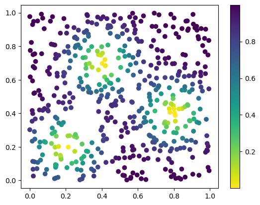
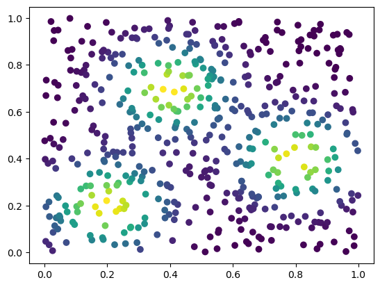
We start from a uniform point cloud, that we will optimize

x = np.random.uniform(size=(500,2))
x = torch.tensor(x, requires_grad=True)
plt.scatter(*x.detach().numpy().T, c=custom_map(x).detach().numpy(), cmap="viridis_r")
plt.colorbar()

<matplotlib.colorbar.Colorbar at 0x7f7c702eae90>

The usual filtration functions (e.g., RipsLowerstar, Cubical, DelaunayLowerstar) automatically detect the differentiability of the input, and propagates the gradient in that case. Nothing changes !

x = np.random.uniform(size=(300,2))
x = torch.tensor(x, requires_grad=True)
from multipers.filtrations import RipsLowerstar, DelaunayLowerstar
# st = DelaunayLowerstar(points=x,function=custom_map(x), flagify=True)
st = RipsLowerstar(points=x,function=custom_map(x))
st.collapse_edges(-1) # litte preprocessing
st.expansion(2)       # adding 2-dimensional simplices are necessary for H1
sm_diff, = mp.signed_measure(st, degree=1, plot=True)
print(sm_diff[0].requires_grad) # Should be true

True

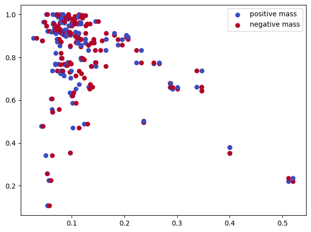
For this example we use the following loss. Given a signed measure \(\mu\), define

\[\mathrm{loss}(\mu) := \int\varphi(x) d\mu(x)\]

where \(x := (r,d)\in \mathbb R^2\) (\(r\) for radius, and \(d\) for codensity value of the original measure) $\(\varphi(x) = \varphi(r,d) = r\times(\mathrm{threshold}-d)\)$

This can be interpreted as follows :

• we maximise the radius of the negative point (maximizing the radius of cycles)

• we minimize the radius of positive points (the edges of the connected points creating the cycles). This create pretty cycles

• we care more about cycles that are close to the mode (the threshold-d part). The threshold is meant to prevent the cycles that are not close enough the the cycles to progressively stop to create loops.

threshold = .65
def softplus(x):
    return torch.log(1+torch.exp(x))
# @torch.compile(dynamic=True)
def loss_function(x,sm):
    pts,weights = sm
    radius,density = pts.T
    density = density
    
    phi = lambda x,d : (
        x
        * (threshold-d)
    ).sum()
    loss = phi(radius[weights>0], density[weights>0]) - phi(radius[weights<0], density[weights<0])
    return loss

loss_function(x,sm_diff) #test that it work. It should make no error + have a gradient

tensor(0.2417, dtype=torch.float64, grad_fn=<SubBackward0>)

As Delaunay complexes are faster to use in low-dimensional Euclidean space, we switch from Rips to Delaunay, and optimize this loss_function.

Another optimization would be to copy the simplextree into a slicer, on which it’s possible to compute a minimal presentation. Computing the Hilbert function is a quite fast computation, so this will not lead to a significative improvement, but consider this optimization when computing harder invariants !

from multipers.filtrations import DelaunayLowerstar
xinit = np.random.uniform(size=(500,2)) # initial dataset
x = torch.tensor(xinit, requires_grad=True)
adam = torch.optim.Adam([x], lr=0.01) #optimizer
losses = []
plt.scatter(*x.detach().numpy().T, c=custom_map(x, threshold=np.inf).detach().numpy(), cmap="viridis_r")
plt.show()
for i in range(101): # gradient steps
    # Little caveat of Delaunay, they are hard to differentiate. 
    # We hence weaken the delaunay complex into a flag complex, which is easier to differentiate, 
    # with the `flagify=True` flag.
    st = DelaunayLowerstar(points=x, function=custom_map(x), flagify=True)
    sm_diff, = mp.signed_measure(st, degree=1)

    # Rips version
    # st = RipsLowerstar(points=x,function=custom_map(x))
    # st.collapse_edges(-1)
    # st.expansion(2)
    # sm_diff, = mp.signed_measure(st, degree=1)
    
    adam.zero_grad()
    loss = loss_function(x,sm_diff)
    loss.backward()
    adam.step()
    losses.append([loss.detach().numpy()])
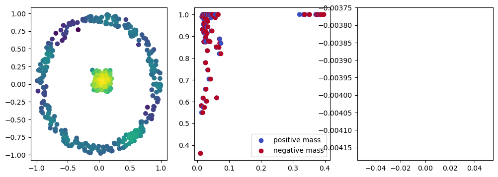
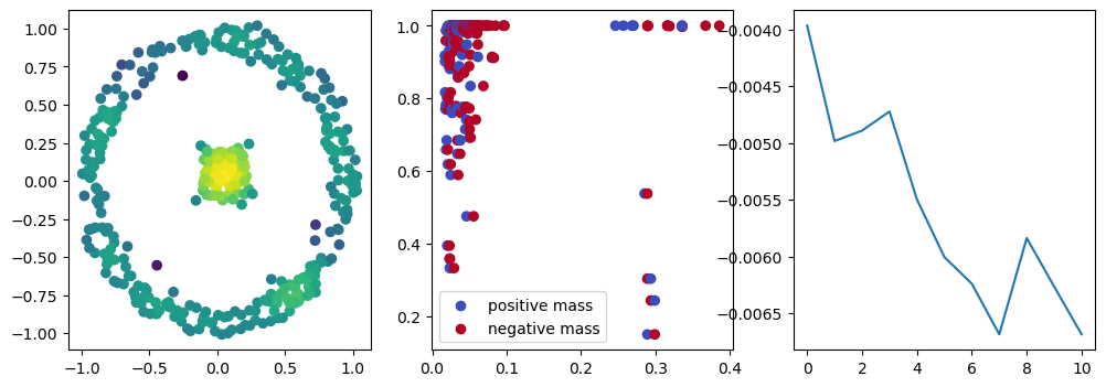
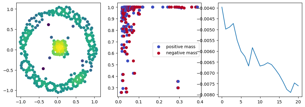
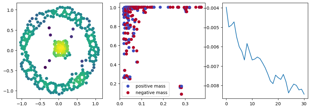
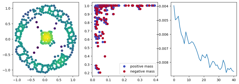
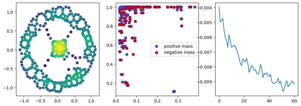
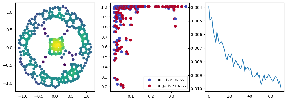
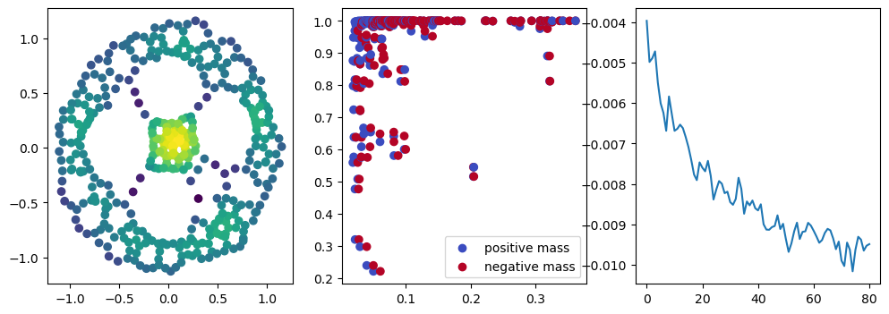
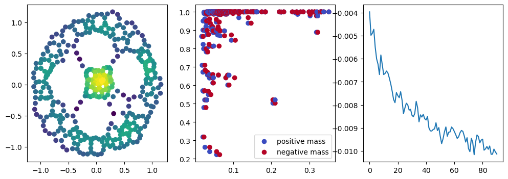
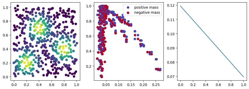
    with torch.no_grad():
        if i %10 == 1: #plot part
            base=4
            ncols=3
            fig, (ax1, ax2, ax3) = plt.subplots(nrows=1, ncols=ncols, figsize=(ncols*base, base))
            ax1.scatter(*x.detach().numpy().T, c=custom_map(x, threshold=np.inf).detach().numpy(), cmap="viridis_r", )
            plot_signed_measure(sm_diff, ax=ax2)
            ax3.plot(losses, label="loss")
            plt.show()
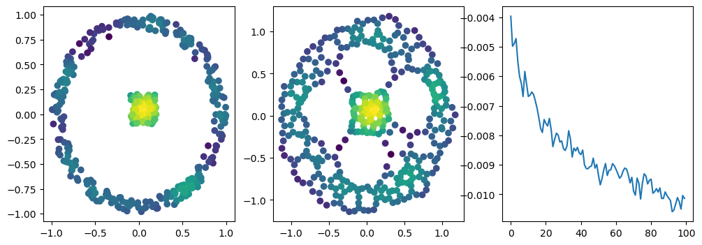
fig, (ax1, ax2, ax3) = plt.subplots(nrows=1, ncols=ncols, figsize=(ncols*base, base))
ax1.scatter(*xinit.T, c=custom_map(torch.tensor(xinit)).detach().numpy(),cmap="viridis_r")
ax2.scatter(*x.detach().numpy().T, c=custom_map(x).detach().numpy(),cmap="viridis_r")
ax3.plot(losses)

plt.show()

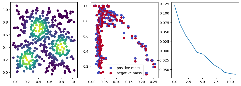
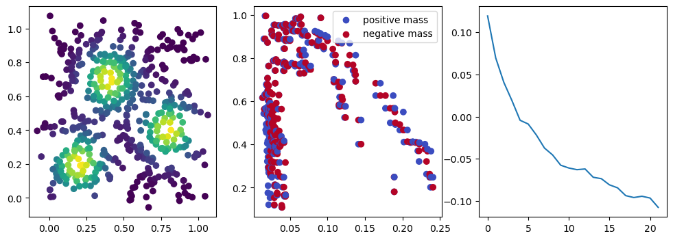
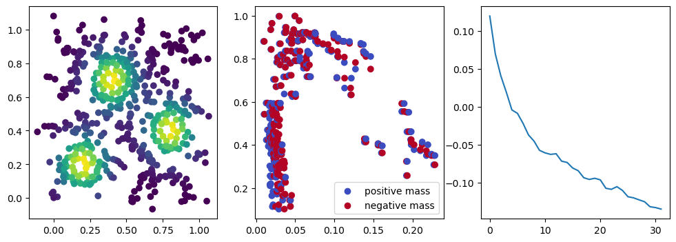
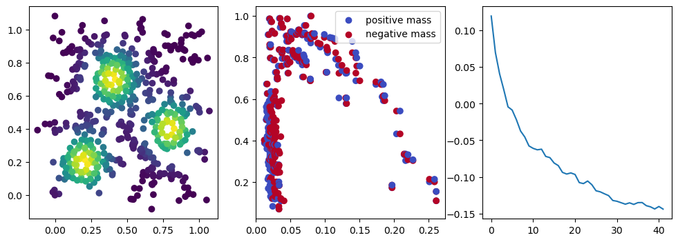
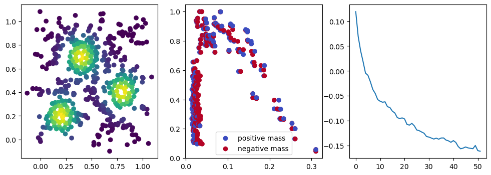
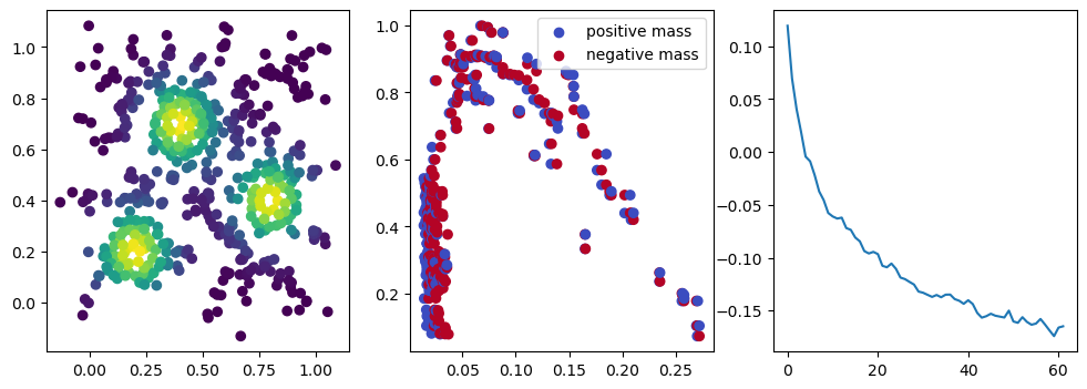
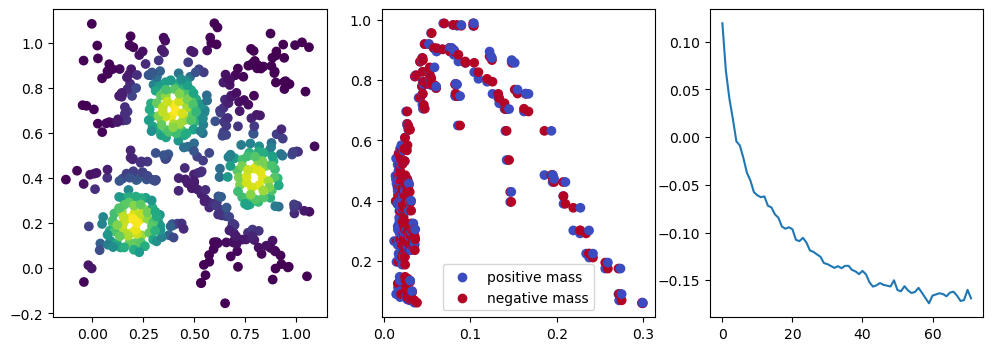
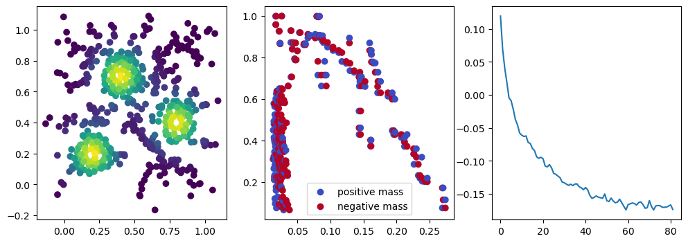
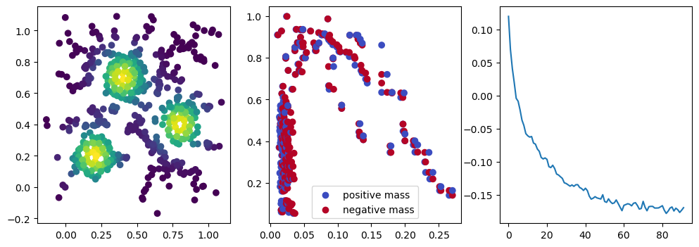
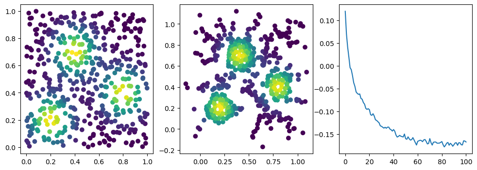
We now observe an onion-like structure around the poles of the background measure.

How to interpret this ? The density constraints (in the loss) and the radius constraints are fighting against each other, therefore, each cycle has to balance itself to a local optimal, which leads to these onion layers.

Density preserving optimization

Example taken from the paper Differentiability and Optimization of Multiparameter Persistent Homology, and is an extension of the point cloud experiement of the optimization Gudhi notebook.
One can check from the Gudhi’s notebook that a compacity regularization term is necessary in the one parameter persistence setting; this issue will not happen when optimizing a Rips-Density bi-filtration, as we can enforce cycles to naturally balance between scale and density, and hence not diverge.

from multipers.filtrations.density import KDE
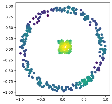
X = np.block([
    [np.random.uniform(low=-0.1,high=.2,size=(100,2))],
    [mp.data.noisy_annulus(300,0, 0.85,1)]
])
bandwidth = .1
custom_map2 = lambda X :  -KDE(bandwidth=bandwidth, return_log=True).fit(X).score_samples(X)
codensity = custom_map2(X)
plt.scatter(*X.T, c=-codensity)
plt.gca().set_aspect(1)

def norm_loss(sm_diff,norm=1.):
    pts,weights = sm_diff
    loss = (torch.norm(pts[weights>0], p=norm, dim=1)).sum() -  (torch.norm(pts[weights<0], p=norm, dim=1)).sum()
    return loss / pts.shape[0]

x = torch.from_numpy(X).clone().requires_grad_(True)
opt = torch.optim.Adam([x], lr=.01)
losses = []
for i in range(100):
    opt.zero_grad()
    st = DelaunayLowerstar(points=x, function=custom_map(x), flagify=True)
    sm_diff, = mp.signed_measure(st, degree=1)
    loss = norm_loss(sm_diff)
    loss.backward()
    losses.append(loss)
    opt.step()
    if i % 10 == 0:
    	with torch.no_grad():
            base=4
            ncols=3
            fig, (ax1, ax2, ax3) = plt.subplots(nrows=1, ncols=ncols, figsize=(ncols*base, base))
            ax1.scatter(*x.detach().numpy().T, c=custom_map2(x).detach().numpy(), cmap="viridis_r", )
            plot_signed_measure(sm_diff, ax=ax2)
            ax3.plot(losses, label="loss")
            plt.show()

with torch.no_grad():
    fig, (ax1, ax2, ax3) = plt.subplots(nrows=1, ncols=ncols, figsize=(ncols*base, base))
    ax1.scatter(*X.T, c=custom_map2(torch.tensor(X)).detach().numpy(),cmap="viridis_r")
    ax2.scatter(*x.detach().numpy().T, c=custom_map2(x).detach().numpy(),cmap="viridis_r")
    ax3.plot(losses)
    plt.show()