Delaunay Lowerstar filtrations

This filtration was introduced by [Delaunay Bifiltrations of Functions on Point Clouds, Alonso et al], whose code is available here.

This bifiltration is very similar to the RipsLowerstar multifiltrations, and is more adapted to low-dimensional Euclidean data.

Definition

Let \(X\) be a point cloud in \(\mathbb R^n\), and \(f\colon X\to \mathbb R\).

The CěchLowerstar bifiltration \(F\) of the point cloud \(X\) , with lowerstar function \(f\) is the bifiltration over \(\mathbb R_+\times \mathbb R\), given by:

\[\begin{align*} \forall (r,d)\in \mathbb R_+\times \mathbb R,\quad& F_{r,d} := \bigcup_{\substack{x\in X \\ f(x)\le d}} B(x,r) \end{align*}\]

The DelaunayLowerstar bifiltration is a 1-critical bifiltration that is topologically equivalent to this one.

An example

import multipers as mp
import matplotlib.pyplot as plt

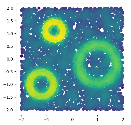
x = mp.data.three_annulus(5_000, 5_000)
f = - mp.filtrations.density.KDE(bandwidth=.1, return_log=True).fit(x).score_samples(x)
plt.scatter(*x.T, c = -f)
plt.gca().set_aspect(1)

[KeOps] Warning : CUDA libraries not found or could not be loaded; Switching to CPU only.

The bifiltration can then be obtained by:

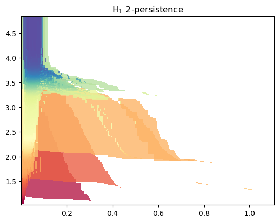
If only a given homological degree is necessary, this construction can made faster:

s = mp.filtrations.DelaunayLowerstar(points=x, function=f, reduce_degree=1)
mp.module_approximation(s).plot()

Autodiff

This bifiltration is not autodiff per se, but can be weakenned into a flag complex to be autodiff w.r.t. the initial point cloud, and the function \(f\).

The gradient is only guaranteed almost everywhere, by [Differentiability and Optimization of Multiparameter Persistent Homology].

import torch
y = torch.from_numpy(x).requires_grad_(True)
f = - mp.filtrations.density.KDE(bandwidth=.1, return_log=True).fit(y).score_samples(y)

st = mp.filtrations.DelaunayLowerstar(points=y, function=f, flagify=True)

Non-problematic operations should preserve gradient

s = mp.Slicer(st).minpres(1)

and invariants should preserve the gradient as well.

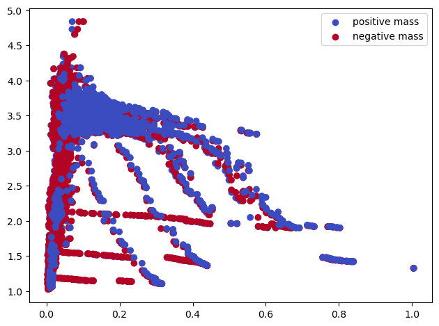
(pts,w), = mp.signed_measure(
    s,
    degree=1, 
    invariant="hilbert",
    plot=True
)
pts.requires_grad # Should be True

True