Representative cycles

Note. This interface is a WIP, and is subject to change.

Invariant computations can be achieved via vineyard computation, which explicitely stores the representative cycles.

We show here how to recover them in python.

import multipers as mp
import matplotlib.pyplot as plt
import numpy as np
import gudhi as gd
import multipers.plots as mpp
np.random.seed(1)

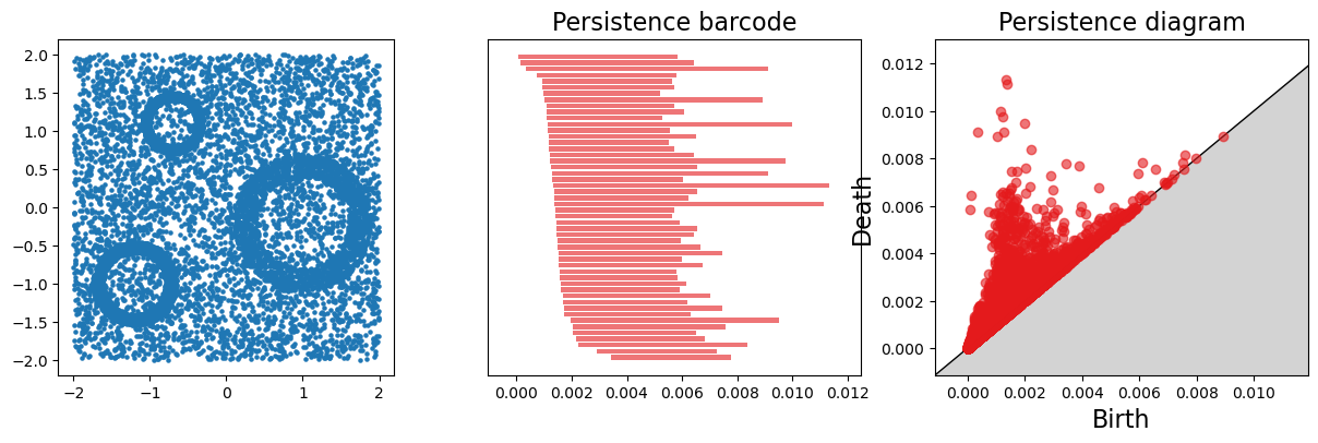
Usual noisy dataset.

np.random.seed(1)
X = mp.data.three_annulus(5000, 5000)
fig, (a,b,c) = plt.subplots(ncols=3, figsize=(15,4))
plt.sca(a)
plt.scatter(X[:,0], X[:,1], s=5); plt.gca().set_aspect(1)
st = gd.AlphaComplex(points=X).create_simplex_tree()
st.compute_persistence()
persistence=st.persistence_intervals_in_dimension(1)
gd.plot_persistence_barcode(persistence=persistence, axes=b, max_intervals=50)
gd.plot_persistence_diagram(persistence=persistence, axes=c)

/Users/dlapous/micromamba/envs/313/lib/python3.13/site-packages/gudhi/persistence_graphical_tools.py:128: UserWarning: There are 9598 intervals given as input, whereas max_intervals is set to 50.
  warnings.warn(

<Axes: title={'center': 'Persistence diagram'}, xlabel='Birth', ylabel='Death'>

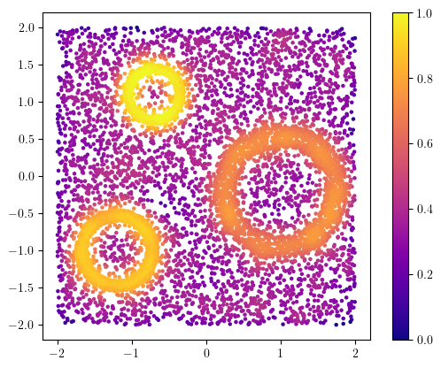
from multipers.filtrations.density import KDE
density = KDE(bandwidth=0.1, return_log=True).fit(X).score_samples(X)
# a bit of renormalization
density -= density.min()
density /= density.max()

# p = np.argsort(-density)
# X=X[p]
# density = density[p]
plt.scatter(X[:,0], X[:,1], s=5, c=density, cmap="plasma")
plt.gca().set_aspect(1); plt.colorbar();

[KeOps] Warning : CUDA libraries not found or could not be loaded; Switching to CPU only.

Filtration

Let’s do a Rips codensity bifiltration

# as we already computed the density, we just need the RipsLowerstar filtration
from multipers.filtrations import RipsLowerstar,DelaunayLowerstar
# Rips
# simplextree = RipsLowerstar(points=X, function = 1-density, threshold_radius=1.5) # this is a simplicial complex

# Delaunay
# Recover id, recover the points id in the simplextree. The indices may be reordered otherwise.
simplextree = DelaunayLowerstar(points=X, function = 1-density, recover_ids=True)

Reduction

# Rips. Edge collpase / expansion do not impact generative cycles recovery
# simplextree.collapse_edges(-1)                             # Removes some unnecessary edges (while staying quasi isomorphic)
# simplextree.expansion(2)                                   # Adds the 2-simplices (necessary for $H_1$ computations)

# minimal presentation's change of basis needs to be recovered. 
# That's `keep_generators=True`, it needs `vineyard=True`
s = mp.Slicer(simplextree, vineyard=True).minpres(1,keep_generators=True)

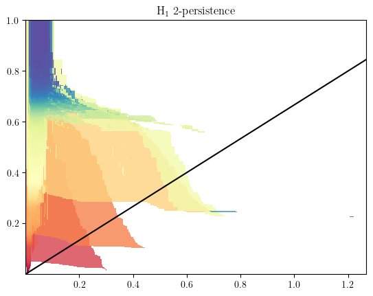
MMA preview

mod = mp.module_approximation(s)

mod.plot()
basepoint = np.array([0,0])
direction=np.array([1.5,1])
slope=direction[1]/direction[0]
plt.axline(basepoint,slope=slope,c="k")

<matplotlib.lines.AxLine at 0x16d1d6660>

Recovering the cycles

We draw the line that intersects the cycles we need to recover, and push s to it. This will fix the vineyard decomposition to this line filtration

s.push_to_line(basepoint=basepoint, direction=direction)

slicer[backend=Matrix,dtype=float64,num_param=2,vineyard=True,kcritical=False,is_squeezed=False,is_minpres=True,max_dim=3]

We can now compute the barcode of degree 1

bc = s.compute_persistence()[1]

And look at which cycles are nontrivial in this line slice

lifetimes = bc[:,1]-bc[:,0] 
idx = np.argwhere(lifetimes>0.01).ravel() # other criterion could be taken

We can then compute representative cycles of these cycles.

cycles = s.get_representative_cycles()[1] #
cycles = [cycles[i] for i in idx]

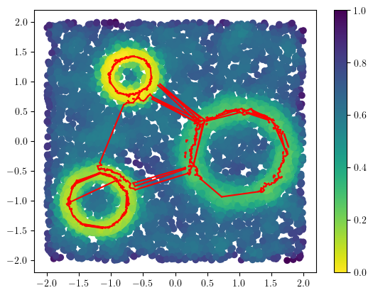
And plot them to double check it.

plt.scatter(*X.T, c=1-density, cmap="viridis_r")
plt.colorbar()

for cycle in cycles:
    cycle = np.array(cycle)
    B = X[cycle[:,0]]
    D = X[cycle[:,1]]
    # plt.scatter(X[:,0],X[:,1], c=density)
    for (a,b) in zip(B,D):
        plt.plot([a[0],b[0]],[a[1],b[1]], c="r")

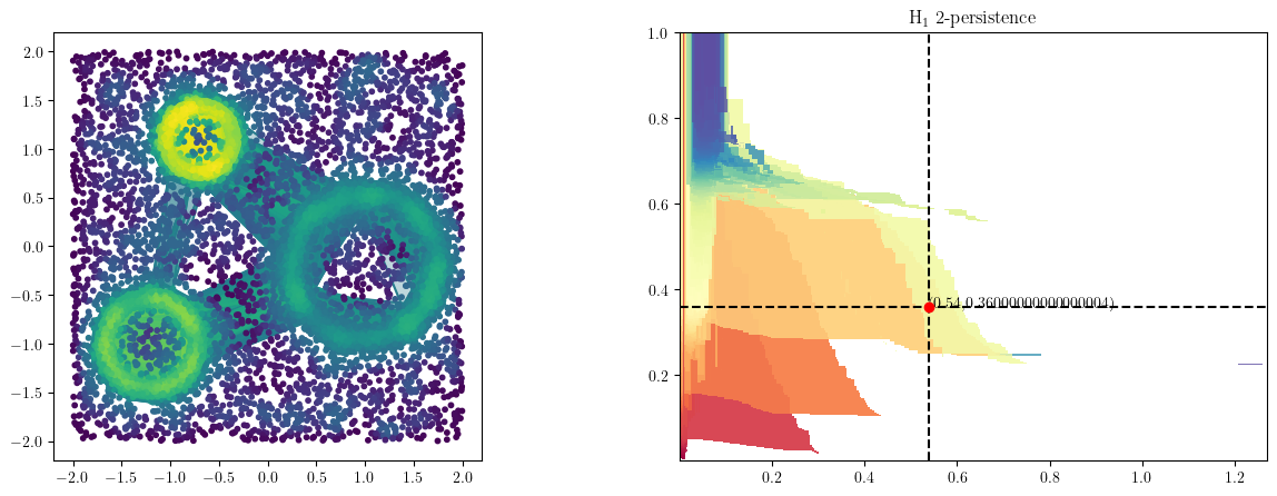
We can also double-check the cycles in the bifiltration.

from multipers.plots import plot_simplicial_complex
t = .54/direction[0]
radius, codens = basepoint + t *direction
plot_simplicial_complex(simplextree, X, radius, codens,mma=mod, degree=1)