Time Series Classification
import multipers as mp
from os.path import expanduser
import pandas as pd
from sklearn.preprocessing import LabelEncoder
from gudhi.point_cloud.timedelay import TimeDelayEmbedding
import numpy as np
import matplotlib.pyplot as plt
np.random.seed(0)
This dataset can be found at https://www.timeseriesclassification.com/description.php?Dataset=Coffee
DATASET_PATH=expanduser("~/Datasets/UCR/")
dataset_path = DATASET_PATH + "Coffee/Coffee"
xtrain = np.array(pd.read_csv(dataset_path+"_TRAIN.tsv", delimiter='\t', header=None, index_col=None, engine='python'))
ytrain = LabelEncoder().fit_transform(xtrain[:,0])
xtrain = xtrain[:,1:]
xtest = np.array(pd.read_csv(dataset_path + "_TEST.tsv", delimiter='\t', header=None, index_col=None, engine='python'))
ytest = LabelEncoder().fit_transform(xtest[:,0])
xtest = xtest[:,1:]
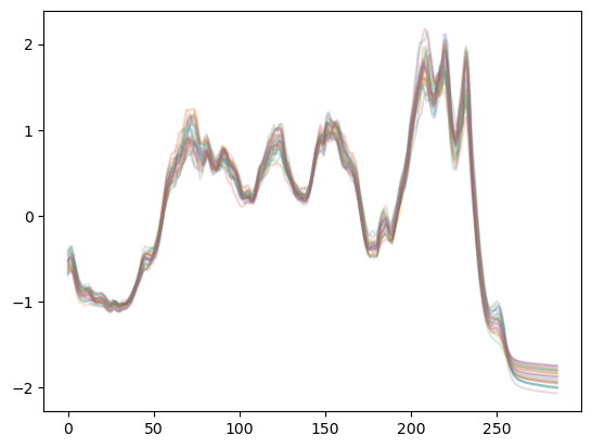
## the time-series of the Coffee dataset
plt.plot(xtrain.T, alpha=.2);
Time Delay Embedding
In this format, time series are not very well suited for a topological analysis.
However, using Time Delay Embedding, which falls into the theory of
Taken’s Theorem
we embed time series into a euclidian space, turning them into curves in a euclidian space.
The advantages of this approach is that this embedding doesn’t depend on reparametrization of the time series,
and its construction doesn’t depend on the number of sampling points.
Furthermore, if the parameters of this embedding are well chosen, the periodicity properties of the time series translates into topological properties of the embedding.
Using the usual Rips-Density bifiltration allows to recover the topological properties (and thus some Fourier coefficients informations) from the time series, as well as their importance (via the density parameter).
Of course, a bunch of reasonable (and faster) multi-filtration can be used instead of this one, e.g., Function-Delaunay.
## Default parameters
dim=3
delay=1
skip=1
TDE = TimeDelayEmbedding(dim=dim, delay=delay, skip=skip)
xtrain = TDE.transform(xtrain)
xtest = TDE.transform(xtest)
np.asarray(xtrain).shape # num_time_series, embedding_curve_sampling, embedding_dimension
(28, 284, 3)
Step by step
This is a point cloud now, so it can be dealt with with usual pipelines.
Here each of entry of xtrain will be turned into two multi-simplextrees :
Rips + (gaussian kernel density estimation with bandwith \(0.1*\mathrm{scale}(\mathrm{xtrain})\))
Rips + (Distance to measure with mass threshold 0.1)
And we’ll see which one gives the best results later.
import multipers.ml.point_clouds as mmp
sts = mmp.PointCloud2FilteredComplex(bandwidths=[-.1], masses=[.1], complex="rips").fit_transform(xtrain)
sts = mmp.FilteredComplexPreprocess(num_collapses=-2, expand_dim=2).fit_transform(sts)
sts[0]
/var/folders/w6/5k5w13s94bq0dfsx2xzqxcsh0000gn/T/ipykernel_71356/1677214221.py:1: DeprecationWarning: multipers.ml.point_clouds is deprecated; use multipers.ml.filtered_complex
  import multipers.ml.point_clouds as mmp
[KeOps] Warning : CUDA libraries not found or could not be loaded; Switching to CPU only.
[SimplexTreeMulti[dtype=float64,num_param=2,kcritical=False,is_squeezed=False,max_dim=2],
 SimplexTreeMulti[dtype=float64,num_param=2,kcritical=False,is_squeezed=False,max_dim=2]]
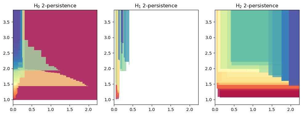
We generate a module approximation for each simplextree
import multipers.ml.mma as mma
mods = mma.FilteredComplex2MMA().fit_transform(sts)
mods[0][0].plot()
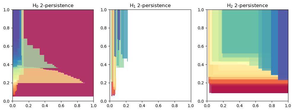
Normalize the filtration values
mods = mma.MMAFormatter(normalize=True).fit_transform(mods)
mod = mods[0][0]
mod.plot()
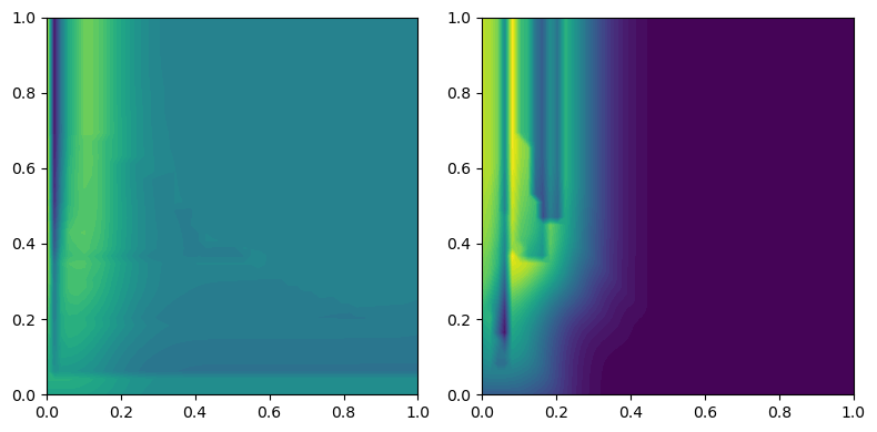
We can then turn these into vectors:
to_img = mma.MMA2IMG(bandwidth=.1, degrees = [0,1], n_jobs = 1, resolution=50, kernel = "gaussian", flatten=False, signed=True).fit(mods)
imgs = to_img.transform(mods)
from multipers.plots import plot_surfaces
plot_surfaces(([np.linspace(0,1,50)]*2, imgs[0][0]), cmap="viridis")
And classify all of this using, e.g., a Random Forest Classifier.
Full pipeline
Note. Although normalization allow for reasonable parameter selection without prior knowledge, it is very recommended to cross-validate the parameters using, e.g., scikit-learn’s GridSearchCV, to significantly increase the performances.
from sklearn.ensemble import RandomForestClassifier
from sklearn.pipeline import Pipeline
## We wrap up everything into this pipeline
pipeline = Pipeline([
    ("st", mmp.PointCloud2FilteredComplex(bandwidths=[-.2], masses=[.1], complex="delaunay")),
    ("preprocess", mmp.FilteredComplexPreprocess(reduce_degrees=[0,1])),
    ("mod", mma.FilteredComplex2MMA(n_jobs=-1)),
    ("normalization", mma.MMAFormatter(normalize=True)),
    ("vectorization", mma.MMA2IMG(bandwidth=.1, degrees = [0,1], n_jobs = -1, resolution=50, kernel = "gaussian", flatten=True)),
    ("classifier", RandomForestClassifier()),
])
# Train step
pipeline.fit(xtrain,ytrain)
Pipeline(steps=[('st',
                 PointCloud2FilteredComplex(bandwidths=[-0.2],
                                            complex='delaunay', masses=[0.1])),
                ('preprocess',
                 FilteredComplexPreprocess(reduce_degrees=[0, 1])),
                ('mod', FilteredComplex2MMA()),
                ('normalization', MMAFormatter(normalize=True)),
                ('vectorization',
                 MMA2IMG(degrees=[0, 1], flatten=True, kernel='gaussian')),
                ('classifier', RandomForestClassifier())])
In a Jupyter environment, please rerun this cell to show the HTML representation or trust the notebook. On GitHub, the HTML representation is unable to render, please try loading this page with nbviewer.org.
Parameters
Parameters
| bandwidths | [-0.2] | |
| masses | [0.1] | |
| threshold | None | |
| complex | 'delaunay' | |
| sparse | None | |
| kernel | 'gaussian' | |
| log_density | True | |
| progress | False | |
| n_jobs | None | |
| fit_fraction | 1 | |
| verbose | False |
Parameters
| num_collapses | None | |
| reduce_degrees | [0, 1] | |
| expand_dim | None | |
| vineyard | None | |
| pers_backend | None | |
| column_type | None | |
| dtype | None | |
| kcritical | None | |
| filtration_container | None | |
| output_type | None | |
| n_jobs | None |
Parameters
| n_jobs | -1 | |
| expand_dim | None | |
| prune_degrees_above | None | |
| progress | False | |
| minpres_degrees | None | |
| plot | False | |
| max_error | -1 | |
| nlines | 557 | |
| from_coordinates | False | |
| complete | True | |
| threshold | False | |
| ignore_warnings | False | |
| direction | None | |
| swap_box_coords | None |
Parameters
| degrees | None | |
| axis | None | |
| verbose | False | |
| normalize | True | |
| weights | None | |
| quantiles | None | |
| dump | False | |
| from_dump | False |
Parameters
| degrees | [0, 1] | |
| bandwidth | 0.1 | |
| power | 1 | |
| normalize | False | |
| resolution | 50 | |
| plot | False | |
| box | None | |
| n_jobs | -1 | |
| flatten | True | |
| progress | False | |
| grid_strategy | 'regular' | |
| kernel | 'gaussian' | |
| signed | False |
Parameters
# Test score
pipeline.score(xtest,ytest)
0.9642857142857143